Background

Consider a simple neural network made up of two inputs connected to a single output unit (Figure 2). The output of the network is determined by calculating a weighted sum of its two inputs and comparing this value with a threshold . If the net input (net) is greater than the threshold, the output is 1, otherwise it is 0. Mathematically, we can summarize the computation performed by the output unit as follows:

Suppose that the output unit performs a logical AND operation on its two inputs (shown in Figure 2). One way to think about the AND operation is that it is a classification decision. We can imagine that all Jets and Sharks gang members can be identified on the basis of two characteristics: their marital status (single or married) and their occupation (pusher or bookie). We can present this information to our simple network as a 2-dimensional binary input vector where the first element of the vector indicates marital status (single = 0 / married = 1) and the second element indicates occupation (pusher = 0 and bookie = 1). At the output, the Jets gang members comprise "class 0" and the Sharks gang members comprise "class 1". By applying the AND operator to the inputs, we classify an individual as a member of the Shark's gang only if they are both married AND a bookie; i.e., the output is 1 only when both of the inputs are 1.

Figure 2: A simple two-layer network applied to the AND problem

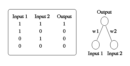
The AND function is easy to implement in our simple network. Based on the network equations, there are four inequalities that must be satisfied:

Here's one possible solution. If both weights are set to 1 and the threshold is set to 1.5, then

Although it is straightforward to explicitly calculate a solution to the AND problem, an obvious question concerns how the network might learn such a solution. That is, given random values for the weights can we define an incremental procedure which will converge to a set of weights which implements AND.

Simple Learning Machines

One of the earliest learning networks was proposed by Rosenblatt in the late 1950's. The task of Rosenblatt's "perceptron" was to discover a set of connection weights which correctly classified a set of binary input vectors.

The basic architecture of the perceptron is similar to the simple AND network in the previous example (Figure 2). It consists of a set of input units and a single output unit. As in the simple AND network, the output of the perceptron is calculated by comparing the net input:

with a threshold (If the net input is greater than the threshold , then the output unit is turned on, otherwise it is turned off).

To address the learning question, Rosenblatt solved two problems. First, it was necessary to define a cost function which measured error. Second, it was necessary to define a procedure which reduced that error by appropriately adjusting each of the weights in the network. However, this requires a procedure (or learning rule) which assesses the relative contribution of each weight to the total error. Rosenblatt decided to measure error by determining the difference between the actual output of the network with the target output (0 or 1). The learning rule that Roseblatt developed based on this error measure can be summarized as follows.

If the input vector is correctly classified (zero error), then the weights are left unchanged, and the next input vector is presented. However, when the input vector is incorrectly classified, there are two cases to consider. If the output unit is 1 when the correct classification is 0, then the threshold is incremented by 1 to make it less likely that the output unit would be turned on if the same input vector was presented again. If the input I_i is 0, then the corresponding weight w_i is left unchanged. However, when the input I_i is 1, then the corresponding weight is decreased by 1 so that the next time the input vector is presented, that weight is less likely to contribute to false classification. On the other hand, when the output is turned off when it should be turned on, the opposite changes are made.

Formally, the perceptron learning rule is defined by two equations. The change in the threshold is given by

where p specifies the presented input pattern, t_p specifies the correct classification of the input pattern, and d_p is the difference between the target and actual outputs. The change in the weights are given by

Exercise 6: Apply the perceptron learning rule to solve the AND problem for w₁ = -0.5, w₂ = 0.5, and = 1.5. Record the weights and threshold after each step of learning, applying the input patterns in the same order as in Figure 2. Make a table of the results. After one step of learning your table should look like:

Input1	Input2	Target	Output	Weight1	Weight2	Threshold
1	1	1	0	-0.5	0.5	1.5
1	0	0	0	0.5	1.5	0.5

How many steps are required to solve the AND problem?

A remarkable property of the perceptron learning rule is that it is always able to discover a set of weights that correctly classifies its inputs, given that the set of weights exists. This important result known as the Perceptron Convergence Theorem (which extends to multiple output networks) fueled much of the early interest in neural networks.

Unfortunately, there are limitations to the types of problems that can be solved by a perceptron.

Why a Hidden Layer?

The limitations of perception were documented by Minsky and Papert in their book Perceptrons (Minksy and Papert, 1969). The now classic example of a simple function that can not be computed by a perceptron (or any two layer network) is the exclusive-or (XOR) problem (Figure 3).

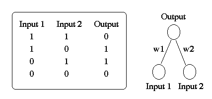
Figure 3: A simple two-layer network applied to the XOR Problem.

A verbal description of the XOR problem (Figure 3) is that the output must be turned on when either of the inputs is turned on, but not when both are turned on. Four inequalities must be satisfied for the perceptron to solve this problem (as was the case for AND):

However, this is obviously not possible since both w₁ and w₂ would have to be greater than while their sum w₁ + w₂ is less than . There is an elegant geometric description of the types of problems that can be solved by a perceptron.

Consider three two-dimensional problems: AND, OR, and XOR. If we represent these problems geometrically (Figure 4), the binary inputs patterns form the vertices of a square. The input patterns 00 and 10 form the bottom left and top left corners of the square and the patterns 01 and 11 form the bottom right and top right corners of the square.

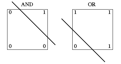
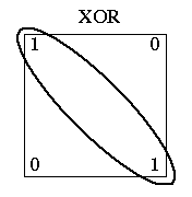
Figure 4: Geometric representation of AND, OR, and XOR.

From a geometrical perspective, the perceptron attempts to solve the AND, OR, and XOR problems by using a straight line to separate the two classes: inputs labelled "0" are on one side of the line and inputs labelled "1" are on the other side. For the AND and OR functions, this is easy to do whereas for XOR it is not. The line separating the two classes is determined by net = . For two-diminensional problems such as AND, OR, and XOR, the line corresponds to

Solving for I₂ yields

In higher dimensions the boundary separating the two classes is a hyperplane

All problems which can be solved by separating the two classes with a hyperplane are called linearly separable. The XOR problem (as presented) is not a linearly separable problem.

However, we can recode the XOR problem in three dimensions so that it becomes linearly separable (Figure 5).

Figure 5: Three-dimensional version of the XOR problem.

In the three-dimensional version, the first two inputs are exactly the same as the original XOR and the third input is the AND of the first two. That is, input3 is only on when input1 and input2 are also on. By adding the appropriate extra feature, it is possible to separate the two classes with the resulting plane. Instead of recoding the input representation, another way to make a problem become linearly separable is to add an extra (hidden) layer between the inputs and the outputs. Given a sufficient number of hidden units, it is possible to recode any unsolvable problem into a linearly separable one.

Exercise 7: Assuming = 1, find a set of weights which solves the 3D version of the XOR problem.

The Credit Assignment Problem in MultiLayer Networks

In the three-dimensional version of XOR network, we showed that a pre-determined extra input feature makes the XOR problem linearly separable. Consider when we add an extra layer to the network instead. The hidden layer provides a pool of units from which features (which help distinguish the inputs) can potentially develop. However, the outstanding question concerns how to learn those features. That is, how can a network develop an internal representation of a pattern?

Since there are no target activations for the hidden units, the perceptron learning rule does not extend to multilayer networks, The problem of how to train the hidden-unit weights is an acute problem of credit assignment. How can we determine the extent to which hidden-unit weights contribute to the error at the output, when there is not a direct error signal for these units. The BackProp algorithm provides a solution to this credit assignment problem.

The Backpropagation Algorithm

The Backpropagation algorithm was first proposed by Paul Werbos in the 1970's. However, it wasn't until it was rediscoved in 1986 by Rumelhart and McClelland that BackProp became widely used.

Feedforward Dynamics

When a BackProp network is cycled, the activations of the input units are propagated forward to the output layer through the connecting weights. Like the perceptron, the net input to a unit is determined by the weighted sum of its inputs:

where a_i is the input activation from unit i and w_ji is the weight connecting unit i to unit j. However, instead of calculating a binary output, the net input is added to the unit's bias and the resulting value is passed through a sigmoid function:

The bias term plays the same role as the threshold in the perceptron. But unlike binary output of the perceptron, the output of a sigmoid is a continuous real-value between 0 and 1. The sigmoid function is sometimes called a "squashing" function because it maps its inputs onto a fixed range.

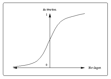
Figure 6: Sigmoid Activation Function

Exercise 8: Calculate the output of the sigmoid function when the net input and bias are zero.

Gradient Descent

Learning in a backpropagation network is in two steps. First each pattern I_p is presented to the network and propagated forward to the output. Second, a method called gradient descent is used to minimize the total error on the patterns in the training set. In gradient descent, weights are changed in proportion to the negative of an error derivative with respect to each weight:

Weights move in the direction of steepest descent on the error surface defined by the total error (summed across patterns):

where o_pj be the activation of output unit u_j in response to pattern p and t_pj is the target output value for unit u_j

Figure 7 illustrates the concept of gradient descent using a single weight. After the error on each pattern is computed, each weight is adjusted in proportion to the calculated error gradient backpropagated from the outputs to the inputs. The changes in the weights reduce the overall error in the network.

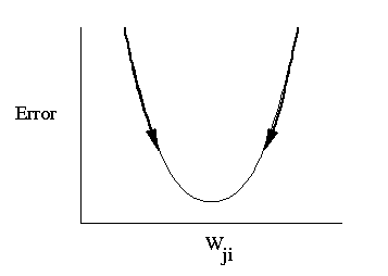
Figure 7: Typical curve showing relationship between overall error and changes in a single weight in a network (reproduced from McClelland and Rumelhart, 1988).

Derivation of the BackProp Learning Rule

In order to derive the BackProp learning rule, we use the chain rule to rewrite the error gradient for each pattern as the product of two partial derivatives. The first partial derivative reflects the change in error as a function of the net input; the second partial derivative reflects the effect of a weight change on a change in the net input. Thus, the error gradient becomes

Since we know what the equation for the net input to a unit is, we can calculate the second partial derivative directly:

We will call the negative of the first partial derivative the error signal:

Thus, the appropriate change in the weight w_ij with respect to the error E_p can be written as

In this equation, the parameter is called the learning rate.

The next (and final) task in the derivation of the BackProp learning rule is to determine what d_pj should be for each unit it the network. It turns out that there is a simple recursive computation of the d terms which can be calculated by backpropagating the error from the outputs to the inputs. However, to compute d_pj we need to again apply the chain rule. The error derivative

can be rewritten as the product of two partial derivatives:

Consider the calculation of the second factor first. Since

The derivative of the sigmoid function has an elegant derivation.

Exercise 9: Demonstrate that the derivative of the sigmoid activation function with respect to the net input simplifies to f(net_pj)(1 - f(net_pj)).

To calculate the first partial derivative there are two cases to consider.

Case 1: Suppose that u_j is an output unit of the network, then it follows directly from the definition of E_p that

If we substitute this back into the equation for d_pj we obtain

Case 2: Suppose that u_j is not an output unit of the network, then we again use the chain rule to write

Combined, cases 1 and 2 provide a recursive procedure for computing d_pj for all units in the network which can then be used to update its weights.

The backpropagation learning algorithm can be summarized as follows. During learning, the weight on each connection are changed by an amount that is proportional to an error signal d. Using gradient descent on the error E_p, the weight change for the weight connecting unit u_i to u_j is given by

where is the learning rate. When u_j is an output unit, then the error signal d_pj is given by case 1 (the base case). Otherwise d_pj is determined recursively according to case 2.

Simulation Issues

How to Select Initial Weights

Now that we waded through all of the details of the backpropagation learning equations, let us consider how we should choose the initial weights for our network. Suppose that all of the weights start out at equal values. If the solution to the problem requires that the network learn unequal weights, then having equal weights to start with will prevent the network from learning. To see why this is the case, recall that the error backpropagated through the network is proportional to the value of the weights. If all the weights are the same, then the backpropaged errors will be the same, and consequently all of the weights will be updated by the same amount. To avoid this symmetry problem, the initial weights to the network should be unequal.

Another issue to consider is the magnitude of the initial weights. When the randomize weights and bias button is activated in BrainWave, all of the network weights and biases are initialized to small random values. What advantage is there in randomized the weights to small values? Reconsider the derivative of the sigmoid activation function. In Exercise 9, we showed that the derivative of the sigmoid is

f'(net_pj) = f(net_pj)(1 - f(net_pj))

Since the weights updates in the BackProp algorithm are proportional to this derivative, it is important to consider how the net input affects its value. The derivative is a maximum when f(net_pj) is equal to 0.5 and aproaches its minimum as f(net_pj) approaches 0 or 1. Thus, weights will be changed most for unit activations closest to 0.5 (the steepest portion of the sigmoid). Once a unit's activation becomes close to 0 or 1, it is committed to being on or off, and its associated weights will change very little. It is therefore important to select small initial weights so that all of the units are uncommitted (having activations that are all close to 0.5 -- the point of maximal weight change).

Local Minima

Since backpropagation uses a gradient-descent procedure, a BackProp network follows the contour of an error surface with weight updates moving it in the direction of steepest descent. For simple two-layer networks (without a hidden layer), the error surface is bowl shaped and using gradient-descent to minimize error is not a problem; the network will always find an errorless solution (at the bottom of the bowl). Such errorless solutions are called global minima. However, when an extra hidden layer is added to solve more difficult problems, the possibility arises for complex error surfaces which contain many minima. Since some minima are deeper than others, it is possible that gradient descent will not find a global minima. Instead, the network may fall into local minima which represent suboptimal solutions.

Obviously, we would like to avoid local minima when training a BackProp network. In some case this may be difficult to do. However, in practice it is important to try to assess how frequently and under what conditions local minima occur, and to examine possible strategies for avoiding them. As a general rule of thumb, the more hidden units you have in a network the less likely you are to encounter a local minimum during training. Although additional hidden units increase the complexity of the error surface, the extra dimensionalilty increases the number of possible escape routes.

The concept of a local minimum can be demonstrated with a very simple network consisting of one input unit, one hidden unit, and one output unit (Figure 8). The task of this network, called the 1:1:1 network by McClelland and Rumelhart (1988), is simply to copy the value on the input unit to the output unit.

Figure 8: The 1:1:1 Network (McClelland and Rumelhart, 1988)

The following exercises explore the concept of local minima using the 1:1:1 network. Even in this simple network, it is possible to have multiple minima and get stuck with a subpar solution.

Exercise 10: To randomize the network weights and biases, select the "Randomize Weights and Biases" button. Now train the network for 200 epochs and record the results under the heading "Simulation 1" in the table below. Record the weight values w1 and w2, the bias values for the hidden and output units, the final error, and whether the network finds a global or local minimum. Finally, describe how your network solved the copy task in this simulation.

Simulation	Minima	Error	w1	w2	bias1	bias2
1.
2.
3.
4.

Exercise 11: For the copy task, it turns out that there are two global minima. Repeat the exercise (possibly more than once) to find an alternative solution. Record the results for the second solution in your simulation table.

So far, we haven't found any local minima in the 1:1:1 network. However, if we freeze the biases on the hidden and output units at zero, we change the system so that instead of two global minima, it now has one local and one global minima (neither of which is optimal).

Exercise 12: Set the Biases on the hidden and output units to zero, and then select BiasUnfrozen for these units Now, rerun to find the local and global minima in the frozen bias version of the 1:1:1 network. Record your results in the table as Simulations 3 and 4.

Learning Rate and Momentum

The Backpropagation algorithm developed in this chapter only requires that the weight changes be proportional to the derivative of the error. The larger the learning rate the larger the the weight changes on each epoch, and the quicker the network learns. However, the size of the learning rate can also influence whether the network achieves a stable solution. If the learning rate gets too large, then the weight changes no longer approximate a gradient descent procedure. (True gradient descent requires infinitesimal steps). Oscillation of the weights is often the result.

Ideally then, we would like to use the largest learning rate possible without triggering oscillation. This would offer the most rapid learning and the least amount of time spent waiting at the computer for the network to train. One method that has been proposed is a slight modification of the backpropagation algorithm so that it includes a momentum term.

Applied to backpropagation, the concept of momentum is that previous changes in the weights should influence the current direction of movement in weight space. This concept is implemented by the revised weight-update rule:

where the subscript n is the learning epoch. With momentum, once the weights start moving in a particular direction in weight space, they tend to continue moving in that direction. Imagine a ball rolling down a hill that gets stuck in a depression half way down the hill. If the ball has enough momentum, it will be able to roll through the depression and continue down the hill. Similarly, when applied to weights in a network, momentum can help the network "roll past" a local minima, as well as speed learning (especially along long flat error surfaces).

In BrainWave, the default learning rate is 0.25 and the default momentum parameter is 0.9. When applying backpropagation to a range of problems, you will often want to use much smaller values than these. For especially difficult tasks, a learning rate of 0.01 is not uncommon.

When to Update Weights

Updating the weights in a BackProp network can be done either after the presentation of each pattern (pattern learning), or after all of the patterns in the training set have been presented (epoch learning). Weights updates in BrainWave are by pattern. If the learning rate is small, there is little differences between the two procedures. However, substantial differences can be observed when the learning rate is large, as the derivation of the backpropagation algorithm assumes that the error derivatives are summed over all of the patterns.

The Development of Internal Representations

Let's now explore how a BackProp network learns to solve the XOR problem.

Figure 9: The XOR Network

Exercise 13: Randomize the weights and biases, and record the output for each of the input patterns. Explain why the output and hidden unit activations are all so similar. Hint: In your explanation refer to the strenghts of the connection weights and how that effects the dynamics of the sigmoid activation function.

Exercise 14: Create a graph of the total error and train the network for 100 epochs. What is the Total Summed Squared (TSS) error after 100 epochs? Continue training the network in 100 epoch steps until the TSS is less than 0.05. Describe the learning curve of the network over the course of training and record the total number of epochs. Note, it is possible that during training your network will get stuck in a local minima. If this happens, re-randomize the weights and start again.

When the network sucessfully learns the XOR task, you should notice that it takes a relatively long time to do so. In fact, it may seem as though the network learns very little during the first several hundred epochs of training,but then accelerates its learning very quickly.

BackProp learning of XOR can be conceptualized as a two stage process. In the first (slow) stage, the network learns to recode the XOR problem so that it is easier to solve. In the slow stage of learning, the network is developing an internal representation of the XOR problem that is linearly separable. Once the XOR problem has been successfully recoded, learning proceeds quickly.

Exercise 15: Record the output and hidden unit activations of the training network for each of the input patterns. How has the network internally represented the XOR problem?

There are different ways to recode the XOR problem so that it is linearly separable. The solution that the network finds depends on the precise values of the initial weights and biases.

So far, we have not considered the effects of changing the learning rate and momentum parameters.

Exercise 16: Try retraining the network with a learning rate of 1.0. Do you see an appreciable change in the speed of learning? What are some possible bad side effects of increasing the learning rate?

Exercise 17: Now try retraining the network after setting the momentum to zero (and the learning rate back to 0.25). You will notice that without momentum, BackProp is much slower to solve the XOR problem. What feature(s) of the error surface might explain this?

Making Predictions: The Jets and Sharks Revisited

Now that you have a more in depth understanding of how BackProp networks learn by example, let's return again to the Jets and Sharks example to address the question of generalization. To do this, we need to examine the ability of a BackProp network to classify input patterns that are not in the training set. If we are confident of a network's ability to correctly classify novel instances, we can use the network to make classification predictions. In the introductory section, we trained a BackProp network to make gang classification judgments. Here, we test its ability to make such judgments for individuals that are not in the training set.

It is easy to imagine a scenario where we have been contracted to develop a reliable method which helps police identify gang members and what gang they belong too. Suppose that to help us devise a method for predicting gang membership, the police have given us access to their database of known gang members and that this database is exactly the data set that we trained the network on.

Consider Table 2 which contains data for four individuals not in the training set. We can imagine that these individuals have recently been arrested and that we have access to their age, education, marital status, and occupation, but not to what gang they belong to. However, in order to help with interrogation, the police need to make an educated guess about whether each suspect is a Jet or a Shark. How do we know whether our network will be a reliable predictor for the police? A simple answer is that we can't know for sure.

Name	Gang	Age	Education	Marital Status	Occupation
George	?	20's	College	Single	Pusher
Linda	?	40's	J.H.	Married	Bookie
Bob	?	30's	H.S.	Divorced	Burglar
Michelle	?	40's	College	Married	Pusher

Table 2: Jets or Sharks?

However, by using the relative activations of the Jets and Sharks units we can make both strong and weak predictions. When the Jet activation is large (near 1.0) and the Shark activation is small (near 0.0), then, the network is making a strong prediction that the suspect is a Jet, whereas the reverse prediction would be made when the Jet activation is smalland the Shark activation is large. In some cases, the network may be unable to make a strong prediction either way (e.g., when both the Jets and Sharks activations are near 0.5).

Each new piece of information added to the database can be compared with the network's predictions to evaluate how well it generalizes. Demonstrating that the network can successfully generalize suggests that it is likely to be a reliable predictor. And with each mistake, we can hopefully use that piece of information to improve the network's performance in future classifications.

The test suite of patterns included in the BrainWave workspace contains the four individuals in Table 2 plus separate test patterns for each characteristic. For example, the 20's input pattern has the 20's unit turned on, and all of the rest of the input units turned off.

Figure 10: Jets and Sharks with a Backpropagation network.

Exercise 18: Train the Jets and Sharks network for 40 epochs and then test the network on George, Linda, Bob, and Michelle. For each, record the output activations in a table and label the network's predictions as "Strong Jet", "Weak Jet", "Strong Shark", or "Weak Shark".

Exercise 19: Use the network to make predictions for the 12 remaining test patterns. The output activation for these patterns is a prediction that an individual is a Jet or a Shark based on only knowing a single piece of information (i.e., what their age OR educational level OR marital status OR occuption is, but not more than one of these.).

Exercise 20: Based on the results from Exercise 19, explain why strong predictions are made for George and Linda. Suppose that we discover that George is a Shark. How does this new piece of information affect your confidence in the model? Would the network be able to easily learn this new piece of data?

Exercise 21: Similarly, explain why weak predictions are made for Bob and Michelle. Would it be more difficult for the network to learn that Bob is a Jet or that Michelle is a Jet.

References

McClelland, J. L. & Rumelhart, D. E. (Eds.). (1988). Explorations in parallel distributed processing: A handbook of models, programs, and exercises. Cambridge, MA: MIT Press.

Rumelhart, D. E., & McClelland, J. L. (Eds.). (1986). Parallel distributed processing: Explorations in the microstructure of cognition (Vol. 1). Cambridge, MA: MIT Press.

---

The Connectionist Models of Cognition homepage.