Using HSGP

Index

• The Context Menu
  • Geographical features
  • Unfolding procedures
  • Colouring
  • Gridlines
• The File Menu

Starting HSGP yields a window resembling the following. On startup, HSGP displays Royal Road, defined over 8 dimensions (4 levels of hierarchy). Clicking in the graph part of the image selects various points (or solutions) in the domain of the function.

The Context Menu

Right-clicking on the graph produces a context menu, shown below.

Geographical Features

The "Highlight" submenu allows you to select which feature of the graph you want to display.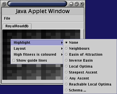

None

No points are highlighted.

Neighbours

Highlights those points that are single-point mutations of the currently selected point (which you can select by left-clicking).

Basin of Attraction

Highlights those points that are "downhill" of the currently selected point. That is, ... .

Inverse Basin

Highlights those points that are "uphill" of the currently selected point. That is, ... .

Local Optima

Highlights the local optima of the function: those solutions for which no single-point mutation produces a fitter solution.

Steepest Ascent

Highlights a path of steepest ascent from the currently selected point to a local optima. If more than one such path exists from a particular solution, a random one will be chosen. Clicking on such a solution multiple times will reveal the range of paths.

Any Ascent

Highlights an ascending path from the currently selected point to a local optima. If more than one such path exists from a particular solution, a random one will be chosen. Clicking on such a solution multiple times will reveal the range of paths.

Reachable Local Optima

Highlights those local optima that are reachable from the current selected point. Not implemented.

Schema ...

Produces a dialog that allows you to define a schema. Points belonging to this schema will be highlighted.

Unfolding Procedures

The "Layout" submenu allows you to select which of two layout algorithms to use.

Recursive

The default layout in which low-order bits correspond to the upper-left, and high-order bits to the lower-right.

Linear

Places the low-order bits on one dimension and the high-order bits on the other.

Mirror

The mirror layout changes the neighbourhood structure of the graph. In the above two layouts, the neighbours of a point are found in the corresponding position across each dimensional `fold' (where the folds are defined by the gridlines). In the mirror layout, the neighbours are located at mirror-symmetric points across the dimensional folds. For example, the top left point and top right point are neighbours.

Colouring

On some occasions it is more useful to have the points of higher fitness drawn in lighter colours and lower fitness drawn in darker colours; on other occasions the reverse is more effective. The "High fitness is coloured" menu allows you to select the colouring strategy.

Black

Points of higher fitness are coloured darker and points of lower fitness are coloured lighter. Points of maximum fitness will be (pure) black and points of minimum fitness will be (pure) white.

White

Points of higher fitness will be coloured lighter than those of lesser fitness.

Gridlines

The "Show guide lines" toggle button turns on and off an overlay of grid-lines. These grid-lines are helpful for orientation, but are less useful in higher dimensions.

The File Menu

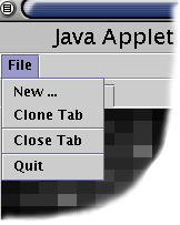The file menu, shown at right, allows new fitness functions to be added, removed, cloned and printed.

New ...

Brings up a dialog which allows you to create a new fitness function.

Clone Tab

Makes an identical copy of the currently selected fitness function, and inserts it after the position of the current function.

Save as PostScript ...

Writes the currently display fitness function to a PostScript file. Not available in applet.

Close Tab

Closes the currently displayed function (destroying it).

Quit

Exits the application.