Methods for representing cost surfaces: Hypercubes and hypergraphs

Hypergraphs are a way of representing all points in a boolean space recursively on a two dimensional display. They are particularly applicable to recursive modular functions. In this section we show how the corners of the n-dimensional hypercube (i.e., the points in the space) are mapped onto the two dimensional graph, and discuss some of the insights that can be gained.

Consider an n-dimensional binary space, {0, 1}ⁿ. Each point in this space is an n-dimensional binary vector, V = (x₀, x₁, ..., x_n-1). The set of all possible points is the set of all possible bit-strings, 000...0 to 111...1. These strings can be represented as the corners of a hypercube. Higher-order hypercubes can be recursively extrapolated from lower-order ones. A three-dimensional space has eight points which can be represented as the corners of a cube. The cube, and its unfolded hypergraph, are shown in Fig.1. In the general case, an n-dimensional space has 2ⁿ points. The corresponding hypergraph is a display of 2^n/2 . 2^n/2 boxes, with each box representing one corner of the hypercube. A sketch of the recursive structure for n = 8 is shown in Fig.2.

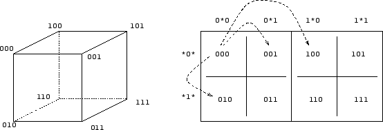
Figure 1: Hypercube and hypergraph. This figure demonstrates the relationship between the cube (left) and its graph form (right), showing the position in the graph to which each point in the cube is mapped. Rows and columns of the graph are labelled by their hyperplane templates. Dotted arrows on the graph show the immediate neighbours of 000.

Formally, using the recursive layout described above, for each n-bit string, B = b_n-1b_n-2...b₀, the cartesian co-ordinates (in binary notation) are given by x = b_n-2b_n-4...b₀ and y = b_n-1b_n-3...b₁. Thus, the lower order bits define the fine structure of the hypergraph and the higher order ones define the gross structure. The string of all zeroes (000...0) maps to the top left corner, and the vector of all ones (111...1) maps to the bottom right corner. The structure of the display can be tuned to the problem under investigation. For example, to keep adjacent dimensions together an alternative layout is to represent the lower order bits on the x-axis, and the higher order bits on the y-axis, corresponding to an alternative unfolding of the hypercube.

Each point in the space has n immediate neighbours, which are the bit strings at a Hamming distance of one. In the graph, these neighbours are located at points 1, 2, 4, ..., 2^n/4 positions away in the same row and column. It is often helpful to overlay grid-lines on the graph which vary in thickness and highlight the recursive symmetries in the graph (see Fig.2).

The regularity of the hypercube connection structure makes it possible to view the hypergraph without explicitly representing the neighbourhood topology. Since the hypergraph is a recursive unfolding of the hypercube, rather than a low-dimensional projection, each corner of the hypercube has a unique position on the graph and no information is lost in the process. Thus, if required, the positions of all connections can be inferred from the position of each string in the hypergraph.

The hypercube has been unfolded onto the hypergraph using translations for each dimension. Hence, recursive symmetries characterise the display. Consider an 8-dimensional space. There are 2⁸ = 256 strings in this space. In GA terms, each allele (0 or 1) in a string defines a hyperplane that divides the space in half. For example, *******1 corresponds to a set of rows and *0****** corresponds to a set of columns. Combinations of alleles such as *0*****1 (also known as clusters) correspond to intersections of the separate hyperplanes.

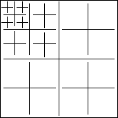
Figure 2: Hypergraph layout for an 8-dimensional space. The 8D hypercube is recursively unfolded to show all 256 strings, with 00000000 in the top left corner, and 11111111 in the bottom right corner.

Given the basic hypergraph layout, we can assign a cost to each point, and plot each point as a coloured box on the hypergraph (see next section for examples). The lower the cost of a particular point (i.e., the more optimal it is) the lighter the colour it is shaded. Thus, points of maximal cost are shaded white, and points of minimal cost are shaded black. The set of points in the hypergraph shows the entire cost surface.

The hypergraph visualisation technique has been implemented as a Java tool which allows several properties of interest to be explored. These include

• the number and distribution of local and global optima (peaks in the landscape)
• points of low fitness, or valleys
• paths from a point to those fitness peaks that can be reached via fitter neighbours (i.e., adaptive walks)
• steepest ascent paths from a point
• basins of attraction for different peaks (the set of points that can climb to that peak)
• (inverse) basins of potential (the set of points that can be reached via an adaptive walk from a point)
• the extent and shape of neutral layers (sets of neighbouring points of equal fitness that provide agents with starting points for exploring different peaks; H-IFF does not exhibit this characteristic).