Visualising H-IFF

Our first example of the hypergraph visualisation approach takes a very simple instantiation of H-IFF, defined over only four dimensions (see Fig.4). The symmetry of the display instantly reveals the symmetry of the underlying function.

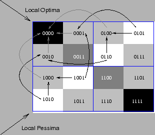
Figure 4: Hypergraph representation for H-IFF defined on four dimensions. Darker shaded areas correspond to points of less cost (i.e., more optimal). Interactions with the visualisation tool reveal that the local optima all fall along the top-left/bottom-right diagonal, and that the points of least fitness (the pessima) fall along the other diagonal. Also shown in this figure are all of the paths of increasing fitness that lead to one of the global optima (0000). The set of points through which these paths travel form the basin of attraction for 0000. The basin of attraction for the other global optimum can be easily derived through the symmetry of the graph.

Examining a hypergraph for a larger space (see Fig.5) shows the generality of the structures observed in Fig.4. The visualisation tool allows some aspects of the cost surface to be directly displayed.

Number of local optima. The local optima can be highlighted, and doing so reveals that they always fall along the diagonal (as observed in the four-dimensional case). Thus, the number of local optima is the square root of the size of the space, 2^n/2. Furthermore, there are an equal number of local pessima (points that have no worse neighbours) which fall along the other diagonal, all of which are global pessima.

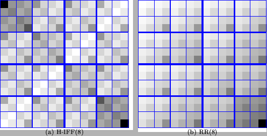
Figure 5: (a) Eight-dimensional H-IFF. As in Fig.4, all local optima fall along the top-left/bottom-right diagonal, and all pessima fall along the other diagonal. Compare the structure of H-IFF with that of Royal Road, shown in (b). The landscape of H-IFF is clearly more complex than that of RR which has only a single fitness peak (at 11111111, in the lower right corner) and which is, effectively, a convex bowl: the basin of attraction for the global optimum is the entire space.

Size and shape of basins of attraction. Some insights can be drawn about the size and shape of the basins of attraction for the local optima, shown in Fig.6. The most obvious observation is that that basin of attraction for the global optimum is a Sierpinski triangle (made more obvious by the manner in which points are highlighted in Fig.6). The recursive structure shows that the size of each basin is given by 3^n/2. Thus, the basins scale in proportion to (the number of points in the Sierpinsky triangle) / (the size of the space), or 3^n/2/2ⁿ = (3/4)^n/2.

Not only does the basin of attraction form a Sierpinski triangle for the global optima, the basins of attraction for local optima are also variants of the Sierpinski triangle (see Fig.6b). Thus, a cursory visual inspection using the hypergraph tool reveals that the basins of attraction for all local optima are of the same size. The size and shape of these basins suggests that random adaptive walks are as likely to terminate at the global optima as they are to terminate at a local optimum (i.e., all outcomes are equally likely). Further detailed analysis revealed that this speculation was indeed correct.

Interactions between basins of attraction. Such a landscape is very difficult to optimise using hill-climbing approaches. The only points in common between the basins of attraction for 00000000 (Fig.6a) and 11111111 (not shown, but symmetric) are the pessima, which lie along the diagonal. In fact, the pessima belong to the basin of attraction for all local optima, or conversely, any local optimum can be reached by an adaptive walk from any pessimum. The separation of the basins at such a low level of fitness indicates a watershed in the landscape that would be difficult to traverse with hill-climbing algorithms. The H-IFF task was designed to be difficult for mutation alone, and the hypergraph makes the success of this design goal directly apparent.

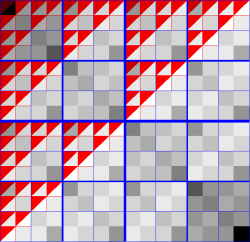
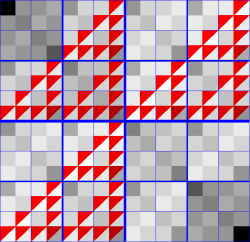
Figure 6:Eight-dimensional H-IFF. Shown are (a) the basin of attraction for the global optimum, 00000000 and (b) the basin of attraction for the local optimum 0011111111 (the bottom right point in the upper left quadrant). Points in the basin have been highlighted by drawing a triangle across the upper left half of the area. (In the interactive tool, the whole square is coloured. The tool was modified to allow display on greyscale media.)