
Tensors are convenient ways of collecting together numbers. For instance, a vector, which is also known as a rank one tensor, could be used to describe the age, gender, and salary of an employee. If Jeff is 50 years old, is male (where male = 0 and female = 1) and earns $56000 per annum then we could describe Jeff with the vector [50, 1, 56000] (see figure 1). Note that vectors (and tensors in general) are ordered. The vector [56000, 1, 50] would describe someone who was 56000 years old who made a total of $50 per annum!

Figure 1: Examples of vectors. (a) a row vector describing Jeff, (b) a column vector, (c) a vector with N components.
The rank one tensor described above has a dimension of three because it contains three components. There is no reason that vectors need be restricted to three dimensions, however. We could have added shoe size, for instance, to increase the dimension to four. Similarly, there is no reason that we need to restrict ourselves to a single row of numbers. A tensor with N rows and M columns is known as an NxM matrix and has a rank of two, indicating that the array of numbers extends in two directions (see figure 2).

Figure 2: Examples of matrices. (a) a 2x2 matrix, (b) a 3x2 matrix, (c) an NxN matrix.
The process of extending the number of directions in which the array extends can theoretically continue indefinitely, creating tensors of rank three, four, five etc. In the following sections, we will look at vectors, matrices and tensors of rank three (see figure 3).
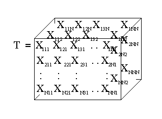
Figure 3: A rank three tensor (NxNxN).
Vectors - Rank One Tensors
Tensors, and in particular vectors, can be represented in
many different forms including:
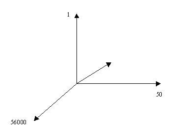
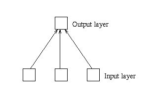
Figure 5: The network corresponding to a vector memory.
The output of this network is defined to be the dot product (or inner product) of the input and weight vectors. A Dot Product is calculated by multiplying together the values which are in the same position within the two vectors, and then adding the results of these multiplications together to get a scalar (see Figure 6a). In the case of the neural network, this involves multiplying each input unit activation by the corresponding weight value and then adding. The dot product of two vectors represents the level of similarity between them and can be extended to higher rank tensors (see figure 6b)
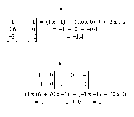
Figure 6: The Dot Product.
The dot product is expressed algebraically as a dot, that is, the dot product of the vectors v and w is written v.w.
Learning occurs in this network by adding the input vectors. Vector addition superimposes vectors of the same dimension. It is calculated by adding together the elements in a particular position in each vector (see Figure 7a). In this way, multiple memories can be stored within the same vector. [Note: the network actually employs Hebbian learning (see Neural Networks by Example: Chapter three). However, when the output unit is fixed at one Hebbian learning is identical to vector addition.]
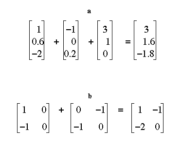
Figure 7: (a) Vector Addition, (b) Matrix Addition.
Again vector addition can be extended to tensors of arbitrary rank (see figure 7b). Vector addition is expressed algebraically as a plus sign (+). So if we wanted to talk about the dot product of v with the addition of w and x we would write v.(w + x). Another useful property to keep in mind is that the dot product distributes over addition. That is:
v.(w + x) = v.w + v.x
Associations are formed using the outer product operation. A outer product between two vectors is calculated by multiplying each element in one vector by each element in the other vector (see Figure 8). If the first vector has dimension d1 and the second vector dimension d2, the outer product matrix has dimension d1xd2. For instance, a three dimensional vector multiplied by a two dimensional vector has dimension 3x2.
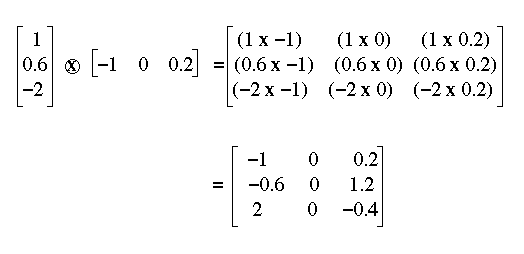
Figure 8: The outer product.
The outer product operation is expressed algebraically by placing the vectors to be multiplied next to each other. So the outer product of v and w is written as v w.
These association matrices are then added into the memory matrix (as in the vector memory case) - so that all associations are stored as a single composite. A matrix memory maps to a two layer network (one input and one output layer) as depicted in Figure 9. The number of input units corresponds to the number of rows in the original matrix, while the number of output units corresponds to the number of columns. Each input unit is connected to each output unit.
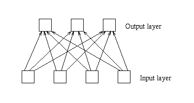
Figure 9: The network representation of a matrix.
Tensors of Rank Three and Above
A tensor of rank three maps to a three layer network (one input layer
with two sets of units, one output layer, and one layer of hidden
units) as depicted in Figure 10. The number of units in the input sets
and the output set correspond to the dimensionality of the tensor. The
number of hidden units corresponds to the number of units in one input
set times the number of units in the other input set. Each hidden unit
has a connection from one input unit from each input set, with a hidden
unit existing for each possible combination. These hidden units are SigmaPi
units, the value of which is set to the multiplication of the two input
units to which it is connected. To implement a rank three tensor, the
weights in the first layer are frozen at one. Consequently, a hidden
unit's activation will equal the multiplication of the activations of
the input units to which it is connected. Each hidden unit is then
connected to each output unit.
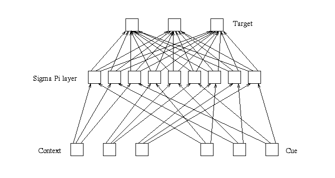
Figure 10: The network representation of a rank three tensor.
In this section, we have been looking at the way in which tensors of
rank one, two and three can be used to store information.
Objective Checklist
The following is a check list of skills and knowledge which you
should obtain while working on this chapter. Go through the list
and tick off those things you are confident you can do. For any item
outstanding, you should refer back to the appropriate section or consult
your tutor.